
 English
 한국어
한국어 中文简体
中文简体Home / News / Industry News / Steinmetz Formula Explained: Coefficients, Fitting and Core Loss Limits
Steinmetz Formula Explained: Coefficients, Fitting and Core Loss Limits
Content
- 1 Typical exponents and what they reveal about a grade
- 2 Fitting Steinmetz coefficients from your own measurements
- 3 Where the formula breaks down: non-sinusoidal flux and pulsed waveforms
- 4 Temperature, DC bias and air gaps: what the coefficients quietly assume
- 5 Specifying a core with Steinmetz data: a practical checklist
- 6 FAQ: Steinmetz formula questions engineers ask
Two power inductors can run at the same 100 kHz switching frequency and the same 120 mT peak flux density, share the same core size, and still differ by a factor of two in core loss. The Steinmetz formula is what lets an engineer predict that difference before the first prototype is built, and it is also the most common reason a thermal calculation comes out wrong: the coefficients inside it are fitted, not derived, and they describe only the window of frequency, flux and temperature in which they were measured.
Pv = k fa Bb
Core loss density expressed as a power law of frequency and peak AC flux density
The Steinmetz formula is an empirical power-law equation that estimates core loss density in a magnetic material from the excitation frequency and the peak AC flux density, using three fitted coefficients: k, the frequency exponent a, and the flux exponent b.
Charles Proteus Steinmetz published the hysteresis law behind this relationship in 1892, after observing that hysteresis loss in iron rose with roughly the 1.6 power of flux density. The modern form keeps that shape and widens it, so one coefficient set covers hysteresis loss, eddy-current loss and excess loss together across a practical frequency band.
| Term | Meaning | Typical unit | Common error |
| Pv | Core loss density | mW per cm3, kW per m3 | Mixing loss per volume with loss per mass |
| f | Excitation frequency | Hz, kHz | Entering kHz while k was fitted in Hz |
| B | Peak AC flux density | T, mT | Using peak-to-peak swing instead of peak |
| k | Material coefficient | Depends on the unit set | Copying k from a different unit system |
| a | Frequency exponent | Dimensionless | Treating a as constant over a wide band |
| b | Flux exponent | Dimensionless | Applying b below the fitted flux range |
Typical exponents and what they reveal about a grade
For commercial soft magnetic materials the frequency exponent a usually falls between 1.0 and 1.8, and the flux exponent b between 2.0 and 3.0, and that pair is a fingerprint of which loss mechanism dominates.
1.3-1.6 Frequency exponent a for Mn-Zn power ferrite, 20 to 300 kHz
2.4-2.9 Flux exponent b for the same grades at room temperature
60-100 C Where many power grades reach their loss minimum
The two exponents are not independent. When a material is hysteresis-dominated, loss scales almost linearly with frequency and steeply with flux, so a sits near 1 and b near 2.5. As frequency rises, eddy currents inside the grains take a larger share, a climbs toward 2, and b flattens. That is why a coefficient set fitted between 20 kHz and 100 kHz can under-predict loss by 30 percent at 300 kHz even when every unit is correct.
| Material family | Frequency exponent a | Flux exponent b | Practical band |
| Mn-Zn power ferrite | 1.3-1.6 | 2.4-2.9 | 20-300 kHz |
| Mn-Zn high-conductivity ferrite | 1.5-1.8 | 2.2-2.7 | 0.3-3 MHz |
| Ni-Zn ferrite | 1.4-1.7 | 2.1-2.6 | 1-30 MHz |
| Powdered iron and soft magnetic composites | 1.1-1.3 | 2.1-2.5 | 20-100 kHz |
| Thin-gauge silicon steel | 1.4-1.9 | 1.8-2.2 | 50-400 Hz |
Read the exponent pair as a fingerprint: b near 2 signals eddy-current-dominated loss, while a near 1 combined with b near 2.5 signals hysteresis-dominated loss.
Fitting Steinmetz coefficients from your own measurements
A usable coefficient set needs at least five flux levels across at least three frequencies measured at one fixed temperature, because three unknowns fitted to three points will reproduce your data exactly and predict nothing.
The sequence below is the one that holds up in practice on Mn-Zn power ferrite and similar materials.
- Fix the boundaries first. Choose a frequency band no wider than one decade, a temperature you can control, and a sinusoidal excitation source.
- Sweep flux density. Take five to seven points from about 20 mT up to the level where the core approaches saturation, spaced roughly evenly in logarithmic terms.
- Sweep frequency at each flux level. Three points per decade is the working minimum, and five is better over a wide band.
- Take logarithms and fit. ln P equals ln k plus a ln f plus b ln B, which is linear in the three unknowns, so ordinary least squares returns them directly.
- Check the residuals rather than the fit quality. If any point inside the window misses by more than about 10 percent, split the window and publish two coefficient sets instead of one.
 Mn-Zn Power Ferrite Cores for Power Conversion DesignBrowse Mn-Zn power ferrite cores by EE, EF, EB, EC, EFD, EI, EM, EPC, EQ, PQ and PTS shapes, with dimensional and AL data.View Product →
Always ask for the fitted window along with the coefficients. A number without a stated range cannot be defended in a design review, and it cannot be compared with a competitor grade.
Where the formula breaks down: non-sinusoidal flux and pulsed waveforms
The original Steinmetz formula assumes a sinusoidal flux waveform, and in a flyback, buck or LLC stage the triangular or trapezoidal flux can push the error past a factor of two.
Original Steinmetz equation
- Assumes sinusoidal flux at a single frequency
- Ignores harmonic content and DC bias
- Fast enough for first-pass sizing and grade comparison
- Safe for mains transformers and near-sinusoidal resonant tanks
Improved generalized Steinmetz equation
- Integrates the time derivative of flux density over one period
- Handles triangular, trapezoidal and discontinuous waveforms
- Needs the same coefficients plus a normalization constant
- Standard choice for PWM converters and gapped inductors
The improved generalized form replaces a single frequency with the actual rate of change of flux, which is what the material responds to.
Pv = (1/T) times the integral over one period of ki |dB/dt|a (delta B)b-a dt
The normalization constant ki is derived from k, a and b so that the equation collapses back to the original form for a sine wave.
On a triangular waveform at 100 kHz, the original equation typically over-estimates core loss by 20 to 40 percent, while the improved generalized form usually lands within about 10 percent.
An intermediate option, the modified Steinmetz equation, replaces the real waveform with an equivalent frequency and reuses the original coefficients. It is easy to implement and reasonable for waveforms with modest harmonic content, but it drifts when the flux carries a large DC bias. The material side of the same problem is covered in this note on how Mn-Zn ferrite reduces core losses.
Mn-Zn High Conductivity Ferrite for High-Frequency ComponentsReview manganese-zinc soft ferrite specifications across EE, EI, EPC, UI, EP, UT, ET and T cores for high-frequency inductors, filters and transformers.View Product →Temperature, DC bias and air gaps: what the coefficients quietly assume
A coefficient set is valid only at the temperature and bias condition where it was measured, and moving from a 25 C bench measurement to an 80 C hot spot can shift the predicted loss by 30 percent or more.
Mn-Zn power ferrites are engineered so that loss reaches a minimum somewhere between 60 C and 100 C. A coefficient set fitted at room temperature therefore over-predicts loss in a running converter, sometimes by a factor of 1.5, and the error changes sign above roughly 110 C.
Three further assumptions matter. DC bias lowers effective permeability, which reduces the AC flux swing for a given applied voltage and therefore reduces core loss while also reducing inductance. An air gap concentrates flux near the gap edges, adding a local loss component that a single loss density figure cannot capture. And a core characterised on a sinusoidal source at low flux will not behave like the same core running saturated in a discontinuous conduction mode converter.
Specifying a core with Steinmetz data: a practical checklist
Treat a coefficient set as a contract: if it does not state units, frequency band, flux range, waveform and temperature, it is not usable for design work.
- Confirm the unit system, including whether k was fitted with frequency in Hz or kHz, flux in T or mT, and loss per volume or per mass.
- Confirm the fitted window, and check that it brackets your operating point with margin rather than sitting at its edge.
- Confirm the waveform assumption, because sinusoidal coefficients applied to a triangular ripple are an approximation, not a calculation.
- Confirm the fitting temperature, since coefficients measured at 25 C are not a substitute for coefficients measured at the winding hot spot.
- Request one verification point at your own frequency and flux, and compare it against your model before committing to a core size.
- Ask about batch consistency, because a small drift in powder chemistry or sintering profile moves k and shows up as unit-to-unit spread in temperature rise.
The strongest supplier answer to a core loss question includes units, fitted frequency band, fitted flux range, waveform, temperature, and a single measured verification point at your operating condition.
Soft Mn-Zn Ferrite Powder YR SeriesExplore YR-series soft magnetic ferrite powders including YR28, YR48, YR48D, YR48B, YR98, YR58 and YR46 grades for selection.View Product →
If the coefficients you were given have no stated window, the fastest route forward is to ask the material supplier for a fitted set at your operating point, with the powder grade and sintering process held fixed.
FAQ: Steinmetz formula questions engineers ask
These four questions come up most often when a coefficient set is being turned into a design or a purchase specification.
What is the Steinmetz formula used for?
It estimates core loss density in a magnetic material from frequency and peak AC flux density. In practice it feeds transformer and inductor design work: comparing grades, sizing a core, estimating temperature rise, and deciding whether a design needs a larger core or a lower-loss material.
What are typical values of a and b for Mn-Zn ferrite?
For Mn-Zn power ferrite measured between 20 kHz and 300 kHz, a commonly falls between 1.3 and 1.6 and b between 2.4 and 2.9. High-conductivity grades used at higher frequency show a closer to 1.7 and a slightly lower b, because eddy-current loss takes a larger share of the total.
Can Steinmetz coefficients be used outside the range they were fitted in?
Not reliably. The equation is empirical, so its coefficients carry no physical meaning outside the window where the regression was performed. Extrapolating one decade beyond the fitted band commonly produces errors of 30 percent or more, and two decades produces numbers that are not worth using.
How do you handle non-sinusoidal waveforms?
Use the improved generalized Steinmetz equation, which integrates the time derivative of flux density over one period, or the modified Steinmetz equation with an equivalent frequency if a simpler implementation is required. The original form is safe only when the flux is close to sinusoidal.
Key takeaway: the Steinmetz formula is a fitted model, not a physical law. Its accuracy depends on how closely your operating point sits inside the fitted window, and on whether your waveform, temperature and bias match the conditions the coefficients were measured under.
Previous Post
No previous article
Next Post
Steinmetz Equation: Reading Core Loss Coefficients for Ferrite Designers